| STARK |
Ribeaud's
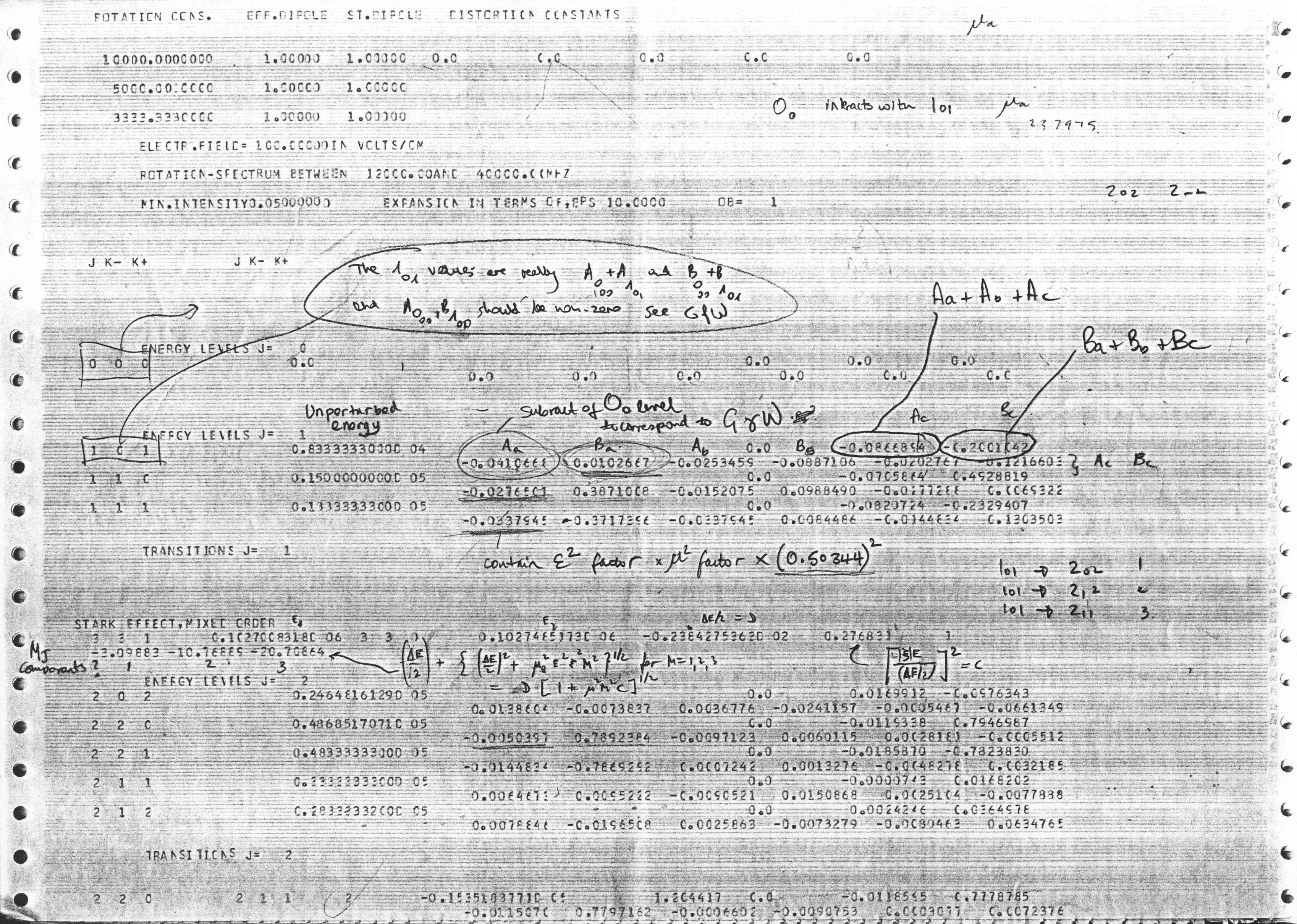
program for Stark coefficients in an asymmetric rotor
|
This
program uses the Golden and Wilson treatment for an asymmetric top
without nuclear quadrupole coupling, J.Chem.Phys. 16,
669 (1948), and as summarized in Gordy&Cook, 3rd ed., pp.468-477.
Stark coefficients for first, second and mixed order components are
calculated if you know how to read the output! The best I can do to
help you is by providing below a scanned version of a hand annotated
copy of the output (from about 1978) that survived in my archives.
NOTE: this program
is kept here for various historical reasons, whereas it is recommended
that the program QSTARK is used for current research applications.
|
 |
| |
| STARK.FOR |
The
listing. A header has been added to the original source, which
explains the structure of the data file. The data is taken from file STARK.DAT and output
is appended to file STARK.RES |
| STARK.DAT |
Test data
for kappa=-0.5
and alpha=0.5
(see the Golden&Wilson paper) |
| STARK.RES |
Results file for the data above,
which can be compared with the Golden&Wilson table of A,B
coefficients. Note that there is a known bug in the coefficients for
the 000 and 101 states. |
| STARK.JPG |
Scanned version of a
hand annotated copy of the output to serve as rudimentary documentation. |
|
|
 |
Back
to the table of programs
| SZK |
Stark
coefficients for an asymmetric rotor
(modification of program STARK by H.M.Pickett)
|
This
is a modified version of the program STARK.F written by H.M.Pickett.
Like its predecessor, SZK is a postprocessing program working on output from the SPFIT/SPCAT package. The program calculates the same quantities as
STARK, but it takes its data from an .STR file produced
by a prior run of SPCAT. The .STR file contains in the second column
the reduced transition dipole matrix element which is equal to the
square root of the linestrength. This is the basis for evaluating the
Golden&Wilson type Stark coefficients as defined in J.Chem.Phys.
16, 669 (1948). The .STR file is
produced by setting STRFLAG in the .INT file to 1 (i.e. the tens digit in the first number in the
top line has to be 1). The output from SZK is written to an .STK file.
Modifications to Pickett's original are as stated at the top of the
listing and have gone mainly into producing what is hopefully
self-explanatory output. Only the coefficients for the energy levels
are calculated so that those for the observed transitions have to be
set up by hand. Note that with this version the coefficients should be
calculated by setting only one of the three possible dipole moment
components to unity - if several components contribute to the Stark
shift then results from two or three such separate runs of SPCAT and SZK
should be combined.
|
|
| |
| SZK.FOR |
The
listing. Input is from files xxx.STR and xxx.INT (the
comment) and the output is written to xxx.STK |
| SZK.EXE |
Executable for Windows |
| SO2.STK |
Specimen
results for SO2 to compare with the Gordy&Cook test
case, p.474 (3rd Ed.). This file is generated by first running SPCAT,
which requires files SO2.VAR and SO2.INT, then running SZK on the results. |
| H2OHF.STK |
Results file for H2O..HF,
which shows the appearance of mixed order output - this can be compared
with J.Chem.Phys. 78, 2910 (1983) |
|
|
|
Back
to the table of programs
| QSTARK |
To fit and to predict
Stark shifts for a rotor with up to one quadrupolar nucleus by direct
matrix diagonalization for each value of the electric field
|
The
incentive for writing this program came from the necessity to deal with
Stark shifts measured in FTMW work on quadrupolar
molecules. The available field strength is quite low so
such shifts fall into the inconvenient intermediate field regime. The
only robust solution is through matrix diagonalization, which has to be
carried out for each combination of field and MF
(the quantisation used is J, K+1, K-1
,F, MF). QSTARK
has been developed from Q2FIT
and irreducible tensor matrix elements for quadrupolar coupling are
from that program. The matrix elements of HE
are from:
H.P.Benz, A.Bauder, Hs.H.Gunthard, J.Mol.Spectrosc.
21, 156 (1966).
An extension of QSTARK to the two quadrupole case is in progress. Note that
most of the internal workings from Q2FIT remain intact, including lack of factorisation so that
matrix sizes and execution times may in some cases become
considerable. Some features:
- Calculation for linear, symmetric, and
asymmetric rotors, with zero or one quadrupolar nuclei
- All of the observed Stark shifts can be
included in one data set (if the field calibration is good enough) -
for example for asymmetric tops without quadrupolar nuclei it is
possible to fit second order and mixed order shifts simultaneously
- The fit can be made either directly to
frequencies or to frequency differences
- It is possible to fit either the effective
electrode separation (calibration) or the dipole moment components and,
if desired, any of the remaining constants in the Hamiltonian - the
latter allows enhanced determination of spectroscopic constants from
Stark shift perturbations
- All types of ΔM transitions can be fitted:
0 and ±1
- Fit can be weighted according to estimated measurement errors
- It is possible to calculate and plot the
behaviour of selected Stark components with the electric field. The
program can produce simple diagnostic ASCII plots in the standard
output file, as well as appropriate files for the gle program, and
thus to obtain higher quality PDF etc. output.
- Experimental measurements can be plotted on
top of predictions (these are placed in a simple two column file of voltages
and frequencies during a fitting run, and this file is reused during a subsequent predictive run)
- It is possible to plot predicted Stark lobe
behaviour as a linear or quadratic function of applied voltage or
electric field
- Separating blank lines and comments can be
embedded between the measured frequencies and will be echoed to the
output if required, and the number of transitions declared in the data
can also be automatically counted by the program
The
recommended paper for citing the the use of QSTARK is:
- Z.Kisiel, J.Kosarzewski, B.A.Pietrewicz,
L.Pszczolkowski, Chem. Phys. Lett. 325,
523-530 (2000).
Known bugs:
The
program calculates correct energies but is known to run into labelling
problems when the off-diagonals in the H matrix become
sufficiently large. Thus indices may be incorrectly assigned to the
eigenvalues. Known instances of such behaviour are:
- first order Stark effects in symmetric tops
- highly perturbing states in asymmetric tops
- high field calculations when μc
is non-zero and QSTARK switches to the complex H matrix formulation
Extensive
dump output, as controlled by the IDUMP parameter, allows checking of
the internal workings in order to obtain a more detailed insight into such
behaviour.
|
|
| |
| QSTARK.FOR |
The
listing. There is much documentation at the top of this listing,
including a detailed description of the input file. The
recommended extension for the input data files is .Q
Compilation:
Compile with any 32-bit compiler,
remembering to use the appropriate option for static allocation of
variables (e.g. -static with f77, or -Qsave with Intel Visual Fortran)
Some compilers (e.g. f77) may treat the
backslash '\' character in strings as a command to generate special
characters. This will affect the proper generation of xtitle
and ytitle lines in the .GLE file. If this is the case replace
'\' by '\\'.
|
| QS.EXE |
Executable for the Windows system..
The program now uses dynamic
dimensioning so it is only limited by the memory available for its
execution.
|
| |
|
| |
Sample fits |
| |
|
| OCS.Q |
Data set for the standard
calibration molecule, set up to determine the electrode spacing. Note
the use of asymmetric rotor quantum numbers, annotations between lines
of the dataset, automatic line counting, and simultaneous fit of ΔM=0
and ΔM=±1
transitions. |
| OCS.RES |
Abbreviated results file for the
above. For supersonic expansion, cavity-FTMW spectroscopy there are
practical limits on the magnitude of the applied electric field so that
Stark shifts are typically less than 1 MHz. This results in only
moderate precision of calibration. |
| |
|
| MECN.Q MEI.Q |
Data sets for the two calibration
molecules used in Warsaw. Larger dipole moments allow measurement of
considerably larger Stark shifts for available electric fields than is
the case for OCS. |
| MECN.RES MEI.RES |
Results files for the above. Note
the improved precision in the determination of the cell constant and
good correspondence between the two determinations. |
| |
|
| ISOX.Q |
The data for isoxazole from
S.McGlone and A.Bauder, J.Chem.Phys. 109,
5383 (1998), in addition to the two dipole components the two poorly
known quadrupole components are to be fitted |
| ISOX.RES |
Results for the above - only an
approximate version of intermediate field analysis was used in the
original paper, and appreciable improvement is apparent. Note
that there are some problems in eigenvalue assignment near line 44 -
the
scheme in the program is over simplistic and fails, it will hopefully
be
improved when a really trying case appears. |
| |
|
| MEIK0.Q |
The MBER data for the J=1←
0 transition in CH3I
from J.Mol.Spectrosc. 160, 351 (1993) - the
paper in which earlier noise in the values of the dipole moment for
methyl iodide was resolved |
| MEIK0.RES |
Results for the above. |
| |
|
| W2HCL.Q |
FTMW data set for (H2O)2H35Cl
consistent with Fig.4 in Chem.Phys.Lett. 325,
523 (2000) |
| W2HCL.RES |
Abbreviated results for the above |
| |
|
| |
Sample predictions |
| |
|
| W.Q |
Data set for (H2O)2H35Cl
similar to W2HCL.Q above adapted to produce the basis for Fig.4 in Chem.Phys.Lett.
325, 523 (2000).
Each of the six bottom lines
specifies a Stark lobe for which calculated points should be generated,
and defines the voltage range, the number of points to be calculated
and the point distribution (whether linear or quadratic). The last line
also defines the Stark shift range of the plots.
|
| EXP.DAT |
The optional data file containing
measured data points to be superimposed on the Stark component plot. |
| W.RES |
The main output file produced by QSTARK from the above
data, containing blocks of calculated points for the Stark components,
as well as a simple ASCII pseudoplot at the bottom.
The same run of QSTARK
also produces files EXPTPLOT.DAT, W.GLE and six files W1.DAT,...,W6.DAT.
|
| W.PS |
The PostScript diagram generated by
running gle
on the data above using the command: gle_ps
w.gle (for gle4.0.7) |
| W1.PS |
The PostScript plot obtained by
changing "The number of iterations" parameter in W.Q above from -2
to -11. In this case the plot is in
portrait orientation and is of frequency against voltage. |
|
|
|
Back
to the table of programs
|