|
The
RECSPE
package described here is the result of a project to
digitise extensive mm-wave rotational spectra of the H2O...HF hydrogen
bonded complex recorded in the Nizhnii Novgorod laboratory in
Russia. Partial analysis of those spectra was published (Belov et al.
J.Mol.Spectrosc. 241 (2007) 124), but the majority of the lines
remained unassigned and only the paper version of those spectra
survived.
In fact the
situation when a spectrum exists only in the form of a paper record and
contains valuable unprocessed information is not that rare. Such
spectra are also often in the form of chart recorder rolls. It
is very desirable to convert such spectra into a digital form that will be
amenable for use with contemporary packages for graphical assignment, such
as AABS.
RECSPE
is a package of programs for conversion into a usable
digital form of such legacy paper spectra. Several graphics programs
(such as Inkscape) can trace a
bitmap image into a vector, which is useful, but the result is still far
from what we would regard as a digital spectrum. The present package
offers a complete route from legacy paper spectra to calibrated digital
spectra in the form of point intensities at a uniform frequency
spacing.
Recovery of paper spectra poses some specific
issues that need to be addressed, and these needed to be dealt with
in the RECSPE
programs:
- Frequency
calibration: This is key to the usability of
recovered spectra. Many old spectra are
inherently nonlinear in frequency. Even if the spectrum was linear
it is possible that nonlinearities may have crept in from uneven
operation of the original recorder or distortions in the paper through
folding or crumpling.
-
Multipage spectra: If the
spectra are in the form of a strip chart record then they need to be
scanned to multiple images that need to be spliced together
The steps in the RECSPE
procedure:
- Scan the spectrum into a reference bitmap
image (300dpi color TIFF with LZW compression is
recommended)
-
Convert the bitmap image to indexed 256
color=8bit 300 dpi BMP, which is the form that will be used for
further analysis. You may also need to modify the scanned
image of the spectrum for optimum tracing and freely available
bitmap graphics programs IrfanView and GIMP are recommended for this
purpose.
-
Use program TRACE to
trace the spectrum from bitmaps to vector representation.
The success of the tracing can be previewed by means of
automatically generated diagrams for the gle package.
-
Use program SPLICE to
splice together traces from adjacent pages of multipage spectra
(you need to ensure that there is sufficient overlap between
their bitmaps).
-
Use program FZERO
to assign a zero order linear frequency scale to
the horizontal axis based on specification of two
characteristic points.
-
Use program MERGE
to combine all spectra into a single
record.
- Use the AABS
package to determine the frequency calibration of
the spectrum and then program
FRECAL
to convert the frequency scale to that resulting
from the calibration.
|
Some of these steps
are only needed for more complex situations. For a single page
spectrum that was plotted linear in frequency you might only need to
use TRACE
and FZERO. For more complex spectra and if you want to achieve
maximum accuracy then you may need to go through the whole procedure,
iterating some steps several times.
Examples of paper
spectra and of their conversion:
Before:
|
After:
|
Stark spectrum of methanol at taken in the 1970's
with the Hewlett-Packard
8460A rotational spectrometer at University College
London:
- meoh_04.jpg =
fourth segment of scanned chart strip output (reduced from
original 11 Mb size) . This strip chart spectrum covers 26.5-40
GHz.
|
meoh_04_uncal.pdf
= result of conversion to pixel coordinates
meoh_04_cal.pdf =
frequency axis added by using FZERO
and pixel coordinates for two widely separated markers, scanned into
a separate marker channel. Note that frequency now increases
from left to right.
|
|
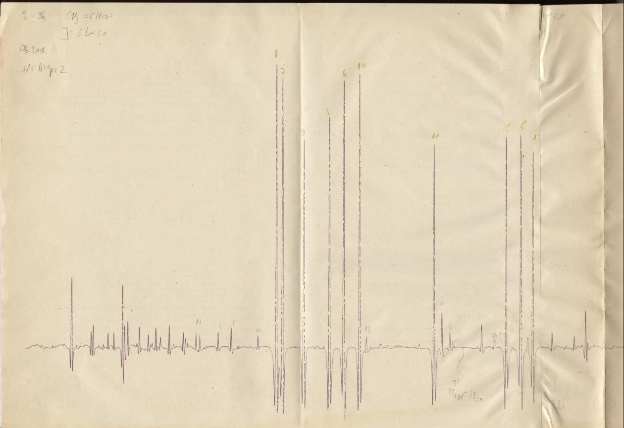
Source modulation spectrum of acrylonitrile at 295 GHz taken in
1986 with the IFPAN spectrometer by free scanning the BWO
source:
- vincn295GHz_a.jpg
= first part of a spectrum glued from several A3 size XY plotter
sheets (this has been reduced from 31 Mb original scan size)
|
vincn295_complete.pdf
= result of conversion using the RECSPE
procedure. The spectrum was self-calibrated since frequencies
of most of the lines are currently well known.
vincn295_zoom.pdf
= zoomed view onto the group of lines preceding the ground state
spline.pdf = the
frequency correction function established for this spectrum
|
|
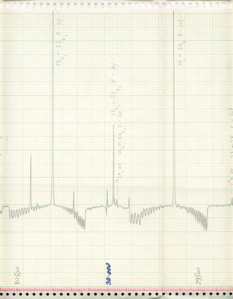
RAD spectrum of H2O..HF at 319 GHz recorded in 1987 in Nizhnii
Novgorod:
- 38a_reduced.jpg =
reduced version of the first scanned sheet of this three sheet
long spectrum. Top trace is H2O...HF, bottom is SO2
reference spectrum.
|
38a_sm.pdf = result of
tracing this spectrum with smoothing
38a_dif.pdf = result
of additional differentiation of the spectrum at the end of
tracing
|
Back to the
table of programs
This is the
key program in the RECSPE
package and it converts a bitmap image of a spectrum into a
string of points. If the spectrum contains a second channel
with markers or a reference spectrum then that channel can also be
analysed synchronously with the main channel. The points are assigned
x,y values in pixel units.
The steps in
using TRACE:
- Scan the spectrum to a lossless bitmap: it is recommended to
use 300 dpi LZW compressed TIFF
-
Convert the bitmap to 8-bit (ie. indexed 256 colour) BMP
standard. Convenient conversion is possible with the batch
convert mode of Irfanview.
-
Establish the RGB colours and their range for the traces of
interest. One or two channel spectra can be traced,
providing the two channels (say spectrum and markers, or sample
and calibration spectra) have been drawn in different
colours). A useful tool for colour identification is
Gimp.
- Gimp, or a similar program may also be used for cleaning up
the spectrum. It is very important that the intensity axis
is true vertical, so that if the image is slanted it should be
rotated. Areas of the image that might confuse the program can be
deleted, examples of these are or edge perforations if their
colour is close to that of the trace.
-
Write the colour values and their tolerances to file
TRACE.INP.
If you do not need the second trace then enter zero values for
its colours. You can also declare whether the traces are
to be smoothed and then optionally differentiated.
NOTE: make sure that the frequency scale, if present
in the spectrum image, is in a very different colour to that of
the spectral trace. If you do not need to convert the
frequency scale then just erase it from the bitmap, otherwise
you may obtain confusing results.
- Run TRACE. You
can view the results directly with gle by clicking on one of the
automatically generated .gle scripts. If
conversion problems are spotted then you might need to retouch
the original bitmap or tune up the TRACE.INP file and redo the
tracing. The gle display will be updated
automatically.
|
The operation
of TRACE
is based on the concept that spectra are single valued
functions so that for a given frequency there should be just one data
point. The bitmap is scanned one column at a time and all pixels in
the specified colour range are identified. The outliers are then
established and rejected, and the y-value of the remaining points
averaged. Interpolation is used for empty columns within the
x-axis range of the
spectrum.
 |
| |
| TRACE.FOR |
Source
listing.
|
| TRACE.EXE |
Windows executable. The program runs
as specified in the trace.inp file. Launch
from the command line in the directory containing the
bitmaps for tracing. Two modes are possible:
- Manual mode: program will trace only
the specified bitmap
- Auto mode: program will attempt to
trace all .BMP files in the current
directory
|
| TRACE.INP |
The control file for TRACE
with entries for tracing the sample bitmap below.
This can be reedited as necessary.
- Colour values are to be established from the bitmap
to be scanned by using the colour picker of any bitmap
graphics program
- If you only want to trace one channel then specify
0 values for RGB colours of trace B
- Traces can be smoothed (recommended) using standard
Savitsky-Golay least-squares polynomial smoothing
- Traces can also be differentiated for use when you
might want to convert from first to second derivative
lineshape. The phase factors ensure upward
central peaks.
|
|
|
| 38A.ZIP |
This is the full bitmap of
the image shown in 38a_reduced.jpg
for the H2O...HF example above.
It is quite large (>8Mb) so it has been
zipped but it can be unpacked and used for
testing
TRACE. |
38A_SM.GLE
38A_SM_A.XY
38A_SM_B.XY
|
One of several sets
of files for gle that will be produced by
TRACE
for the bitmap above. The .XY files are the
resulting traces while various additional files allow
convenient viewing of the results of the tracing. The
files are produced in sets for the raw traces, smoothed
traces, and differentiated traces (if specified).
These three files correspond to the gle diagram
shown in 38a_sm.pdf.
The .XY
traces are ASCII files containing in the first two columns
the x,y values that will be used for
further processing. The last two columns list actual
pixel coordinates of the points (top-left corner of bitmap
is 0,0) for direct comparison with coordinates displayed by
most graphics programs.
The .XY
files can be read and displayed with the SVIEW_L
program of the AABS package.
|
|
|
 |
Back to the RECSPE
summary
| SPLICE |
SPLICing of
traces for multipage spectra
|
This program splices traces for adjacent scanned pages of multipage
spectra by aligning the overlap regions. So it is necessary to
exercise some foresight during the scanning process to ensure that there is
sufficient overlap between adjacent pages.
The use of the QGLE
previewer from the gle package is mandatory in this case.
Once the package is installed, and SPLICE is
launched then all you need to do is to click on the automatically generated
file SPLICE.GLE to view
the splicing for the current parameters.
|
| |
| SPLICE.FOR |
Source
listing.
|
| SPLICE.EXE |
Windows executable. The program is to be
launched from the command line in the directory containing
the traces. For the input file as below you will see the
following
screen. At the same time a file SPLICE.GLE is generated
and you need to click on that in order to preview the
splicing with QGLE.
After these preliminaries you need to manually hunt around
for the best splicing parameters, by typing in the option
number and its value. |
SPLICE.INP
|
The control file. This can be reedited as necessary
and the entries shown are for the sample case below.
If you specify only one channel conversion and generic
file names MOLNAM and
MOLNAM1
then SPLICE
expects to find files MOLNAM.XY and
MOLNAM1.XY.
If two channel conversion is specified then
SPLICE
expects to find MOLNAM_A.XY
+ MOLNAM_B.XY
and MOLNAM1_A.XY
+ MOLNAM1_B.XY.
The first block of the splicing options controls
the QGLE display, while the last
three parameters control the splicing. The crucial
aligning parameter is the
x-axis overlap width
but you may also need to change the other two
parameters. Once you are satisfied that optimum splicing
has been reached you need to exit SPLICE by
pressing ENTER, when the parameters in SPLICE.INP
will be updated. The contents of
this file underneath the top block will be copied over so
that commenting/previous versions of parameters can be
kept there.
|
|
|
38a_dif_a.xy
38a_dif_b.xy
38b_dif_a.xy
38b_dif_b.xy
|
The traces for spectrum
38a (channel a and b) and for spectrum 38b (channel a and
b) to be spliced using the input file above
|
| SPLICE.PDF |
Illustration of the
display that you will see in the QGLE viewer of gle on
launching SPLICE with
the data above. You can see that there is some
x-axis
misalignment that can be corrected by changing the value of
parameter number
6.
|
38ab_a.xy
38ab_b.xy
|
The traces resulting from
optimum splicing of the data above, channel A is SO2,
channel B is H2O...HF.
|
|
|
|
Back to the
RECSPE
summary
| FZERO |
Assignment of zero order
frequency axis
|
This program
assigns the frequency axis to a trace, which can be either directly
from TRACE, or result from splicing with SPLICE.
Frequency is recalculated in a straightforward linear conversion based on
coordinates of two points. For a spectrum that is known to be
nonlinear this is really a zero order operation to make subsequent handling
easier. If the spectrum is linear then this may be all that you need
to do.
You need to load the traced
spectrum into SVIEW_L and
measure two lines (or features) to determine their X-coordinates for use in calibration.
These X-coordinates and the known
true frequencies of these two points are then to be written to the file
MOLNAM.FPT, where
MOLNAM is the generic name
used for files associated with this spectrum.
|
| |
| FZERO.FOR |
Source listing.
|
| FZERO.EXE |
Windows executable, to be used from the
command line. The program will:
- first try to convert file
MOLNAM.XY
(single channel mode).
- if there is no MOLNAM.XY then the program will try to convert
files MOLNAM_A.XY
and MOLNAM_B.XY
(two channel mode)
|
|
|
MEOH04_SM.XY
|
Uncalibrated trace for the example
methanol spectrum as shown in meoh_04_uncal.pdf |
| MEOH04_SM.FPT |
The file with the two calibration points
for the above.
|
| MEOH04_SM.SPE |
The resulting file corresponding
to meoh_04_cal.pdf |
|
|
| 38ab.FPT |
The file
with the two calibration points for the H2O...HF+SO2
example discussed in the description of SPLICE. |
38ab_a.SPE
38ab_b.SPE |
The files resulting from
addition of the zero order frequency axis to files 38ab_a.xy and 38ab_b.xy from the SPLICE
example
|
|
|
|
|
|
Back to the
RECSPE
summary
This program
merges all traces with assigned frequency scale into a single spectrum. The
operation is as follows:
- frequency sorted list of basic properties spectra in
the current directory is produced
- the spectra are unified to a common frequency grid
(defined by the internal parameter FSTEP) and each spectrum
SPECNAM.SPE is converted
to U_SPECNAM.SPE
- all U_
spectra spectra are then merged into two files, U_A.SPE containing
all A channel spectra, and U_B.SPE
containing all B channel spectra.
|
| |
| MERGE.FOR |
The source
listing. |
| MERGE.EXE |
Windows executable to be launched from the
command line in the directory containing the spectra.
Note that:
- spectral files are to have
extension .SPE and are to be
in the two column ASCII standard as produced by
FZERO
- no spaces are allowed in file
names
- data points have to be equidistant
in frequency
- missing parts are filled with
zeroes, overlapping parts are connected at the middle
of the overlap region
|
| LIST |
Listing of the spectra
found and processed by MERGE. This file
is identical in format tho the LIST file required by
the AABS package for
displaying the ranges of spectra available for
analysis.
This listing summarises all constituent spectra from the
H2O...HF project that were combined into one single
spectrum. |
u_A.spe
u_B.spe
|
The result of operation of
MERGE
on files
38ab_a.SPE and
38ab_b.SPE
obtained above with FZERO.
The files were converted to the 0.5 MHz frequency grid and
if more spectra were available then those would have been
merged into these two output files.
|
|
|
|
Back to the RECSPE
summary
| FRECAL |
FREquency
CALibration of a spectrum
|
This program
calibrates the frequency axis of the spectrum by applying a correction
based on a cubic spline function fit to a predefined set of calibration
points. Alternatively, a previously determined spline function can be
used, providing that it was determined for the same frequency axis (for
cases when a separate reference channel was recorded).
A prerequisite
to running this program is to produce a file of frequency calibration
points. For this you need to use the AABS package. The
spectrum is to be displayed in SVIEW_L and the
predictions with true frequencies of lines should be displayed displayed
in ASCP_L.
The two program should be in linked mode ensured by the presence of
a suitable SVIEW_L.INP file in the working
directory. You need to declare MOLNAM.FRE as the
name of the fitting data file, where MOLNAM is
the generic name for the project. Calibration
measurements should then be written to that file with the
F8
option of ASCP_L.
|
| |
| FRECAL.FOR |
The source
listing. |
| FRECAL.EXE |
Windows executable to be run from
the command line. The only parameter that you
specify is the generic name, MOLNAM, for the
files in question. The program then expects that
you have the file FRECAL.INP (as below)
and have prepared:
- MOLNAM.SPE =
the file containing the spectrum to be calibrated (in
the IFPAN binary format, as written with the
m option of SVIEW_L)
- MOLNAM.FRE =
the file with the calibration points produced with the
F8 option of ASCP_L
operating in linked mode with SVIEW_L.
Alternatively if a run such as that described above
has taken place on a reference spectrum and you have an
identically recorded sample spectrum to calibrate then
you can reuse the spline function MOLNAM_spline.FNC
generated in the previous run by copying it to a file
where the MOLNAM part of
the name corresponds to that used for the sample
spectrum.
The primary output file will be MOLNAM_frecal.SPE.containing
a two column ASCII version for the spectrum for the same
points as in the input spectrum, but with frequency of
each point recalculated according to the calibration
function. This point spacing in this spectrum will
NOT be equidistant in frequency, so you can convert to
equidistant frequency spacing with SVIEW_L
|
| FRECAL.INP |
The control file for
FRECAL.
In the presence of noise affecting the calibration points a
simple cubic spline function fit may not be the
optimum solution. You therefore have the option of
interpolating additional points that will reduce spline
function excursions, and also of smoothing the correction
function. The best solution is to use a mixture of
these techniques.
|
|
|
| A.SPE |
Spectrum for the SO2 channel in H2O...HF
spectra used as a worked example for the complete
RECSPE
procedure. This file is a direct conversion to binary
format made with SVIEW_L
of spectrum u_A.spe obtained above with
MERGE. |
| A.FRE |
The calibration points for
this spectrum determined by using the AABS
package with spectrum A.SPE, as above, and
linelists for SO2 from the CDMS
database. Linelists for the ground states of the
parent and isotopic species, and for the bending satellite
in the parent were loaded.
The calibration points do not have to be in any particular
order, but FRECAL will
sort them in frequency.
|
A_FRECAL.SPE
|
The main result of
operation of FRECAL on
the two files above (without the use of interpolation and
smoothing). This is a frequency calibrated spectrum
in ASCII standard. The file also contains an
additional third column listing the original
frequencies. Note that the points in this
spectrum are NOT equidistant in frequency but this spectrum
can be read and converted to equal frequency increments
with SVIEW_L |
A.GLE
A_calpts.out
A_spline.out
|
Additional files produced
by of FRECAL that
allow viewing of the spline function used for the
calibration. Spline functions are powerful tools but
are susceptible to experimental errors in declared
points. The sensitivity is particularly high for
points very close together and it is recommended that a
check for unexpected spline function excursions is
made.
|
| A_spline.pdf |
The spline function
diagram produced with the 'export' option of QGLE
from the three files above. The lowest and highest
frequency points have zero correction because they
were already calibrated, in the process of defining the
zero order frequency scale in FZERO.
|
B.SPE
B_spline.fnc
|
The two files necessary for calibration of the spectrum
in the H2O...HF channel:
- the file B.SPE is a binary
version of u_B.spe obtained above
with MERGE.
It is necessary to ensure that the first point in this
spectrum is at the at the same frequency as in the
reference spectrum.
- the file B_spline.fnct is a
binary file containing the spline function that was
generated during calibration of the SO2 channel.
It is just a copy of the file A_spline.fnc
generated during that operation.
|
| B_FRECAL.SPE |
The frequency calibrated
H2OHF spectrum at 321GHz.
|
|
|
|
Back to the RECSPE
summary
|
 package
for:
package
for: