|
This work deals with misfit angles, which are observable
in ferroelastic phase transitions. In the literature the misfit angles were
calculated for six different ferroelastic phase transitions, where there is
only one possible misfit angle. In this work the method for obtaining all
misfit angles (for the cases where there is more than one possible) is
introduced. Also the expressions for all possible misfit angles for each
ferroelastic species are given.
|
1. Introduction
In a ferroelastic structure, several ferroelastic domain states can be
formed [1]. These states have the same crystal structure and differ only in
the orientation with respect to the coordinate system of the paraelastic
phase. Since all domain states are energetically equivalent, they can coexist
in the same crystal. The ferroelastic domains and domain walls can be well
observed in a polarized-light microscope [2]. When only a single domain is
formed in the ferroelastic structure, its single domain state has a prominent
crystallographic orientation, and is referred to as the ideal domain
state. In a multi-domain structure the orientations of the domain states
differ from the orientations of the corresponding ideal domain states.
The domain walls between two ferroelastic domains that satisfy the conditions of the strain compatibility are then referred to as permissible domain walls. These domain walls must contain all directions for which the change in length of any infinitesimal vector of the prototype, due to spontaneous strain, is equal in the two adjacent domains [1]. If the existence of a permissible domain wall between two domains is possible, then there are always two planes in which the permissible domain walls can be formed. Furthermore, these two planes are always perpendicular to each other [1]. If the permissible domain walls cannot exist, then the two domain states will join only when external stress is applied. The boundaries between the two domain states are then not well-defined planes, often irregular, curved or diffuse, with internal stresses and dislocations. In this work we will consider only the cases when a permissible domain wall can be formed.
To form a domain wall between two ferroelastic domains a certain rotation of the corresponding ideal domain states of the adjacent domains is necessary [3, 4]. The aim of this work is to calculate all possible angles, the so-called misfit angles, at which the ideal domain states could be rotated in order to form the permissible domain wall. The magnitude of these angles depends on the spontaneous strain and on the relation between the two domain states. In Ref. [4] the angles have been calculated for six different phase transitions. In this work, these calculations are performed for all possible ferroelastic phase transitions.
2. Spontaneous strain tensor
The spontaneous strain tensor is defined in such a way that the volume of the
prototype does not change after the spontaneous strain, although in reality
the volume changes due to thermal expansion. The spontaneous strain tensor
accounts only for the change in the crystal structure. This condition is
expressed in the following formula [5]:
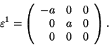
As is shown in Ref. [6] the form of the spontaneous strain tensor depends only on the groups of symmetry P of the prototypic phase and E of the ferroelastic phase, respectively. Then we define the F-operations as the operations that are in P but not in E. The F-operations represent the symmetries that were lost in the phase transition. Any domain state of the ferroelastic structure has all the symmetries of the group of symmetry E. The F-operations transform one domain state into the other domain states. Tables for the forms of spontaneous strain tensors for all domain states for each ferroelastic phase transition can be found in Ref. [7].
Generally, there is more than one operation that transforms one certain domain state S1 into another domain state S2 (the quantities for different domain states are denoted by superscripts behind the symbols of the quantities). If one of the F-operations is a mirror plane or a twofold axis, then this plane, or the plane perpendicular to the twofold axis is going to be the W permissible domain wall, because it satisfies all the conditions. The W' wall is going to be perpendicular to the W wall. The exact orientation of the W' wall depends on the exact values of the components of the spontaneous strain tensor [1].
While calculating the misfit angle of the ideal domain states the spontaneous
strain difference tensor ![]() is introduced. It is defined as the
difference of the spontaneous strain tensors of two different domain states
is introduced. It is defined as the
difference of the spontaneous strain tensors of two different domain states
The spontaneous strain tensor possesses the point inversion as a symmetry
element and therefore the spontaneous strain tensors have the same form for
all crystal classes belonging to the same Laue's group, since the classes
differ only in the point inversion symmetry. From this one can conclude that
it is not necessary to perform calculations for phase transitions between all
possible crystal classes, but only for the 11 Laue's groups. Therefore, we
need to perform calculations for only one of the crystal species
corresponding to this phase transition and the result is valid for all other
species that exhibit the same phase transition. For example, for the phase
transition from Cubic 1 to Tetragonal 1 we have three possible ferroelastic
species:
![]() . If we take for example the
species with the highest symmetry, which is the m3mF4/mmm transition, the
calculations would be the same for the other two species.
. If we take for example the
species with the highest symmetry, which is the m3mF4/mmm transition, the
calculations would be the same for the other two species.
3. Calculation of the misfit angle
The misfit angle ![]() is the whole angle that the two domains have to
rotate at in order to join in a permissible domain wall (see Fig. 1).
is the whole angle that the two domains have to
rotate at in order to join in a permissible domain wall (see Fig. 1).
![\includegraphics[width=7cm]{ino1}](img8.gif)

3.1. Geometrical approach
Let us show an example of calculating the misfit angle ![]() using
geometrical methods. Let us consider the case of the species 4/mmmFmmm.
using
geometrical methods. Let us consider the case of the species 4/mmmFmmm.
In Ref. [7] we can find the form of the spontaneous strain tensor for the
first domain state
The point with the coordinates in the prototypic structure [x,y,z] is
displaced to the point with the coordinates [x',y',z'] in the ferroelastic
structure. These coordinates in both domain states can be expressed in terms
of x,y,z and the spontaneous strain tensors
As we can see from this result, in the direction of the z axis there is no
mechanical strain. Therefore we will limit our considerations to the plane
z=0. For our calculation it is best to consider a square lying in the plane
that has its centre in the origin, and the sides parallel to the axes x,y,
respectively. This square will be deformed into a rectangle. The whole
situation is shown in Fig. 1. The centre of the square has coordinates
[0,0,0] and the coordinates of the upper right vertex are [1,1,0]. From the
calculations above we get the coordinates of the point in the first domain
state [1-a,1+a,0] and in the second domain state [1+a,1-a,0]. From the
figure, it follows that
The geometrical approach can hardly be generalized and can lead to many
difficulties, e.g. in the case of Cubic ![]() Trigonal transition,
when the trigonal axis is parallel to [111]. In fact the example shown above
is probably the simplest case of a phase transition. Therefore we need to
find a more general way of calculating the misfit angle. In the next section
the algebraical approach is discussed in detail.
Trigonal transition,
when the trigonal axis is parallel to [111]. In fact the example shown above
is probably the simplest case of a phase transition. Therefore we need to
find a more general way of calculating the misfit angle. In the next section
the algebraical approach is discussed in detail.
3.2. Algebraical approach
Let us consider the spontaneous strain tensor ![]() for the first
domain state and
for the first
domain state and ![]() for the second domain state. Now we will
assume that there can exist a permissible domain wall between these two
domain states. Let us consider an arbitrary vector x that lies in the
domain wall. The elongation of this vector after the spontaneous strain in
the individual domain states is (in Einstein's notation)
for the second domain state. Now we will
assume that there can exist a permissible domain wall between these two
domain states. Let us consider an arbitrary vector x that lies in the
domain wall. The elongation of this vector after the spontaneous strain in
the individual domain states is (in Einstein's notation)
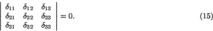
For very small deformations, which is our case, the misfit angle of the domain states is given as the eigenvalue of the spontaneous strain difference tensor.
The eigenvalues ![]() of the spontaneous strain difference tensor
of the spontaneous strain difference tensor ![]() can be found as solutions of the secular equation
can be found as solutions of the secular equation
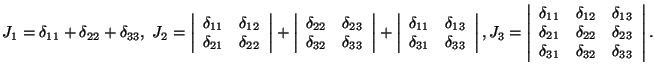 In our
case, the equation will be simplified, since J1=0 according to (3) and J
3=0 according to (15). Equation (16) then takes on the following form:
In our
case, the equation will be simplified, since J1=0 according to (3) and J
3=0 according to (15). Equation (16) then takes on the following form:
3.3. Calculating all possible angles for a phase transition
Using the above method, all possible misfit angles for all ferroelastic phase
transitions were calculated. For each ferroelastic phase transition one must
take all pairs of domain states. For each domain pair, it is necessary to
calculate the spontaneous strain difference tensor, check if the determinant
was zero, and if so, then calculate the misfit angle using the formula (19).
In the list of results, all species belonging to the phase transition, the
spontaneous strain for the first domain state and all possible misfit angles
are listed for each phase transition.
As an example, let us consider the phase transition Tetragonal 2 ![]() Triclinic. The spontaneous strain tensors for the four possible domain
states are as follows:
Triclinic. The spontaneous strain tensors for the four possible domain
states are as follows:
Now let us evaluate the spontaneous strain difference tensor for all possible
pairs
Only the cases of domain pairs S1, S3 and S2, S4 yield a zero determinant.
For these pairs we get the same result and the only possible angle for this
type of phase transition
4. List of results
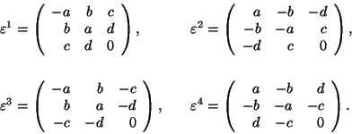
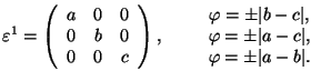
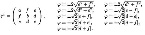
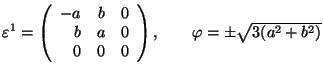
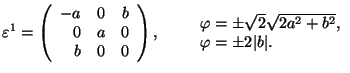
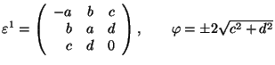
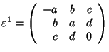
Cubic 1 ![]() Tetragonal 1
Tetragonal 1
![]() cubic axes; in S1, the tetragonal axis (ferr.)||x
cubic axes; in S1, the tetragonal axis (ferr.)||x
 .
.
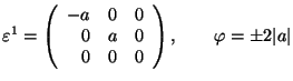
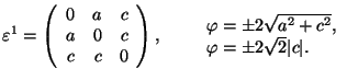
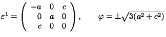
Cubic ![]() Trigonal
Trigonal
![]() cubic axes; in S1, the trigonal axis (ferr.)||[111]
cubic axes; in S1, the trigonal axis (ferr.)||[111]
 .
.
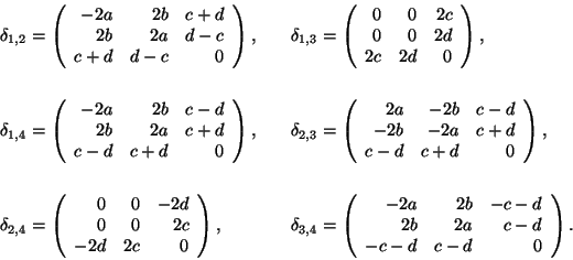
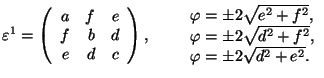
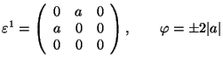
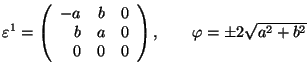
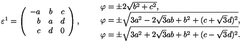
Cubic 1 ![]() Orthorhombic
Orthorhombic
![]() cubic axes
cubic axes
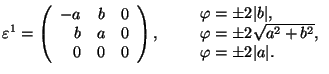
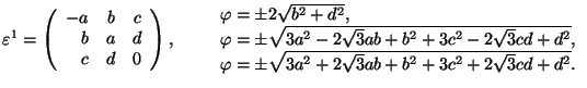
Cubic 1 ![]() Orthorhombic
Orthorhombic
![]() cubic axes; in S1, the orthorhombic axis (ferr.)||x
cubic axes; in S1, the orthorhombic axis (ferr.)||x
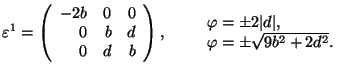
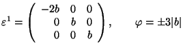
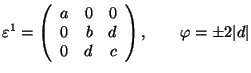
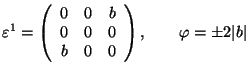
Cubic 1 ![]() Monoclinic
Monoclinic
![]() cubic axes; in S1, 2 (ferr.)||x
cubic axes; in S1, 2 (ferr.)||x
Cubic 1 ![]() Monoclinic
Monoclinic
![]() cubic axes; in S1, the monoclinic axis
cubic axes; in S1, the monoclinic axis![]()
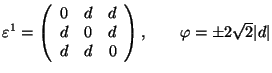
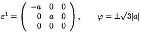
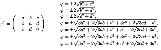
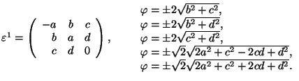
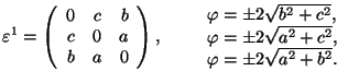
Cubic 1 ![]() Triclinic
Triclinic
![]() cubic
axes
cubic
axes
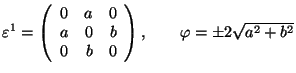
Cubic 2 ![]() Orthorhombic
Orthorhombic
![]() cubic axes
cubic axes
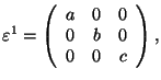 no permissible domain walls.
Cubic 2 ![]() Monoclinic
Monoclinic
![]() cubic axes; in S1, 2
(ferr.)||x
cubic axes; in S1, 2
(ferr.)||x
 .
.
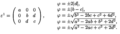
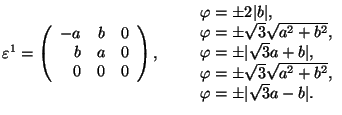
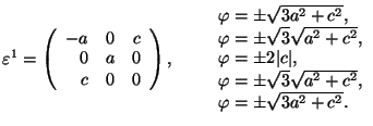
Cubic 2 ![]() Triclinic
Triclinic
![]() cubic axes
cubic axes
Hexagonal 1 ![]() Orthorhombic
Orthorhombic
![]() 6 or
6 or ![]() or
or ![]() ; in S1, x||the orthorhombic axis
(ferr.)
; in S1, x||the orthorhombic axis
(ferr.)
 .
.
Hexagonal 1 ![]() Monoclinic (P)
Monoclinic (P)
![]() 6 or
6 or ![]() 2 or
2 or ![]()
Hexagonal 1 ![]() Monoclinic (
Monoclinic (
![]() or
or ![]() 2 or
2 or ![]() ; in S1, y||the monoclinic axis (ferr.)
; in S1, y||the monoclinic axis (ferr.)
Hexagonal 1 ![]() Triclinic
Triclinic
![]() 6 or
6 or ![]() , x||2 or
, x||2 or ![]() ; in S1, x||the hexagonal axis (ferr.)
; in S1, x||the hexagonal axis (ferr.)
Hexagonal 2 ![]() Monoclinic
Monoclinic
![]() 6 or
6 or ![]()
 .
.
Hexagonal 2 ![]() Triclinic
Triclinic
![]() 6 or
6 or ![]() 2 or
2 or ![]()
 .
.
Tetragonal 1 ![]() Orthorhombic (P)
Orthorhombic (P)
![]() 4 or
4 or ![]() the orthorhombic axis (ferr.)
the orthorhombic axis (ferr.)
 .
.
Tetragonal 1 ![]() Orthorhombic (S)
Orthorhombic (S)
![]() 4 or
4 or ![]() 2 or
2 or
![]() the orthorhombic axis (ferr.)
the orthorhombic axis (ferr.)
 .
.
Tetragonal 1 ![]() Monoclinic (P)
Monoclinic (P)
![]() or
or ![]() 2 or
2 or ![]()
Tetragonal 1 ![]() Monoclinic (
Monoclinic (
![]() or
or ![]() 2 or
2 or ![]() ; in S1, y||the monoclinic axis (ferr.)
; in S1, y||the monoclinic axis (ferr.)
Tetragonal 1 ![]() Monoclinic (
Monoclinic (
![]() or
or ![]() 2 or
2 or
![]() the monoclinic
axis (ferr.)
the monoclinic
axis (ferr.)
Tetragonal 1 ![]() Triclinic
Triclinic
![]() or
or ![]() or
or ![]()
Tetragonal 2 ![]() Monoclinic
Monoclinic
![]() 4 or
4 or ![]()
 .
.
Tetragonal 2 ![]() Triclinic
Triclinic
![]() or
or ![]()
 .
.
Trigonal 1 ![]() Monoclinic
Monoclinic
![]() or
or
![]() ; in S1, y|| the monoclinic axis (ferr.)
; in S1, y|| the monoclinic axis (ferr.)
 .
.
Tetragonal 1 ![]() Monocpage
Trigonal 1
Monocpage
Trigonal 1 ![]() Triclinic
Triclinic
![]() 2 or x
||2 or
2 or x
||2 or ![]()
Trigonal 1 ![]() Triclinic
Triclinic
![]() 2 or
2 or ![]()
Trigonal 2 ![]() Triclinic
Triclinic
![]() 3
3
 , no
permissible domain walls.
, no
permissible domain walls.
Orthorhombic ![]() Monoclinic
Monoclinic
![]() the orthorhombic axes; y|| the monoclinic axis (ferr.)
the orthorhombic axes; y|| the monoclinic axis (ferr.)
 .
.
Orthorhombic ![]() Triclinic
Triclinic
![]() the
orthorhombic axes
the
orthorhombic axes
Monoclinic ![]() Triclinic
Triclinic
![]() 2 or
2 or ![]()
 .
.
5. Conclusion
The aim of this work was to calculate the misfit angles of domain states
joining in a permissible planar domain wall, which satisfies all the
conditions of mechanical compatibility. The explicit formulae, giving the
result as a function of the spontaneous strain tensor for the first domain
state, have been derived for all 30 possible types of ferroelastic phase
transitions, in which the compatible domain wall can be formed. In the cases,
where there are more than two possible ferroelastic domain states, all
different pairs of domain states have been investigated. For six types of
phase transitions the results correspond with the results obtained by
Shuvalov et al. [4]. For the remaining 24, the explicit formulae for the
misfit angles have not been published before.
Acknowledgments
The author would like to express many thanks to his advisors Prof. Vaclav
Janovec and Dr. Zdenek Kluiber for their discussions, ideas, time and help.
The author also wishes to thank his fellow-student Petr Chaloupka for
spending a lot of time helping with this work. Finally, many thanks go to
Prof. Henryk Szymczak for his help with the preparation of this material for
publishing.
References
1. J. Sapriel, Phys. Rev. B 12, 5128 (1975)
2. H. Schmid, E. Burkhardt, E. Walker, W. Brixel, M. Clin, J.-P. Rivera, J.-L. Jorda, M. Francois, K. Yvon, Z. Phys. B, Condens. Matter 72, 305 (1988)
3. V. Janovec, D.B. Litvin, L. Richterova, Ferroelectrics 157, 75 (1994)
4. L.A. Shuvalov, E.F. Dudnik, S.V. Wagin, Ferroelectrics 65, 143 (1985)
5. J.F. Nye, Physical Properties of Crystals, Clarendon, Oxford 1960
6. J.C. Toledano, Ann. Telecommun. 29, 249 (1974)
7. K. Aizu, J. Phys. Soc. Jpn. 28, 706 (1970)