This paper was awarded in the I International Competition (1992/93) "First Step to Nobel Prize in Physics" and published in the competition proceedings (Acta Phys. Pol. A 85 Supplement, S-7 (1994)).
The paper is reproduced here due to kind agreement of the Editorial Board of "Acta Physica Polonica A".

DYNAMICS OF EARTH CLIMATE EVOLUTION

D.R. Bitouk

Kolmogorov's School of the Moscow State University
Kremenchugskaya str., 11, Moscow, Russia

In this paper we discuss some properties of the dynamics of the Earth climate. Using the method of pseudo phase space for the Time Series of paleoclimatic data, we measure the Kolmogorov entropy and the fractal dimension values of the Earth's global climate system. We also discuss the global climate prediction.
PACS numbers: 92.60.Ry, 05.45.$+$b

1. Introduction

In recent years many attempts have been made in order to investigate the Earth's global climate evolution. On the basis of the observations, made with the help of the $\delta$O$^{18}$ content's isotope analysis in a deep-sea core [1, 2] it has been established that during the last million of years sequence of ice-ages took place on the Earth, lasting nearly 100000 years each. Therefore, during last million years the climatic system evolution may be regarded as transitions between two different regimes: ice-age climate and the climate, which is close to the modern one. So far, both factors, which are responsible for these transitions, and their dynamics are unknown.

Although a number of theoretical studies of global climate were successful, still there are problems with modelling the climate dynamics [7]. Those problems are mainly related to too large number degrees of freedom in dealing with models, which makes it impossible to study their dynamics.

2. Reconstruction of the climatic system dynamics from the Time Series of the paleoclimatic data

Almost all methods of the analysis of the system dynamics assume that the number of state variables, necessary to describe the system dynamics, is given. It is clear that those methods cannot be used to study the climatic system, because number of significant modes, contributing to the system dynamics is unknown a priori.

One of the ways to deal with the climate dynamics is based on the analysis of the structure of the system's phase space. If, as time goes on, the system reaches the steady state, then it should be displayed in the convergence of the phase trajectories to the invariant set in the phase space, which is called ``attractor'' [4].

The fractal dimension of the attractor provides us with the information about the character of the system's dynamics.

Climate oscillations during the last million years can be considered as those which reached the steady state. Therefore, to find out the characteristics of the dynamics of the climatic system it is necessary to determine the attractor dimension, which, in its turn, needs the analysis of the phase trajectories. To find out the climate attractor dimension the method of the reconstruction of the system dynamics from the Time Series can be used.

This suitable method has been recently developed by Grassberger and Procaccia [3, 4] and it has been used to study the dynamics of a number of complicated physical processes.

The method consists in following. Let $X(t)$ be the Time Series of one of the system variable. Let us obtain the set of arrays from $X(t)$ by shifting its values by a fixed lag $\tau$ ( $\tau=l\Delta t$, where $l$ is an integer value, $\Delta t$ is a time interval between step-by-step sampling). Selecting from the Time Series $K$ equidistant points, the following set of the digital variables is obtained:

$$Y_1=\left[ X(t_1), X(t_2),\ldots, X(t_K)\right],$$

$$Y_2 =\left[ X(t_1+\tau), X(t_2+\tau), \ldots ,X(t_K+\tau)\right],$$

$$\qquad\qquad\qquad\dots$$

$$Y_N=\left[X(t_1+(N-1)\tau), X(t_2+(N-1)\tau), \ldots,X(t_K+(N-1)\tau)\right].$$

The given number $N$ of digital variables $Y_1,\ldots,Y_N$ determines some phase space, which is known as pseudo phase space of the considered system. The given space consists of $k$ points

$$Z_i =\left[X(t_i),X(t_i+\tau), \ldots, X(t_i+(N-1)\tau)\right].$$ (1)

The connection between phase and pseudo phase space of the system is given by Takens' theorem [4, 5]. Let us deal with the pseudo space, which is of $2d+1$ dimension, where $d$ is the phase space dimension. Takens' theorem declares that this pseudo phase space metric characteristics are equivalent to the metric characteristics of the system phase space (the distances in both spaces are related by a coefficient, which is uniformly limited and differs from zero).

However, the dimension of the phase space for the climatic system is unknown. This problem can be easily solved by the following method. Let us construct the pseudo phase spaces of increasing dimensions and find the one in which some of its characteristics (such as, for instance, the fractal dimension of attractor) reach the asymptotic values. This pseudo phase space may be considered as satisfying Takens' theorem [3].

Using Takens' theorem, one can easily prove that if the system phase space dimension is $d$ and the dimension of the pseudo phase space is $2d+1$ then the fractal dimensions of two attractors put in both phase spaces are equal to each other [3].

Hence, we arrive at the following algorithm. Consider the set of $K$ points of the form (1) in the pseudo phase space of $N$ dimensions. Let us introduce a vector notation $\vec{Z}_i$. A reference point $\vec{Z}_i$ from these data is now chosen and distances $\vert\vec{Z}_i-\vec{Z}_j\vert$ to each of the remaining points are computed. This allows us to count the data points that are within a prescribed $r$; one arrives at the quantity

$$C(r)={1\over K^2} \sum^K_{i\not=j} H\left( r-\vert\vec{Z}_i -\vec{Z}_j\vert\right),$$ (2)

where $H(s)$ is the Heaviside function, $H(s)=0$ if $s<0$, $H(s)=1$ if $s>0$.

This quantity measures the extent to which the presence of a data point $\vec{Z}_i$, affects the position of the other points. $C(r)$ may thus be referred to as the integral correlation function of the attractor.

In Refs. [4, 6] it is proved that the fractal attractor's dimension $D$ is the inclination of $\ln C(r)-\ln r$ dependence plot.

As it has been already said, the fractal dimension of system attractor can be obtained as the asymptotic value of the fractal dimension of the attractor put in the pseudo phase space. It was proved [4, 6] that if the dimension $D$ reaches the asymptotic value, then evolution of system may be considered as an example of the deterministic dynamics, because noise does not show tendency to reach an asymptotic value.

It is commonly known that much of our information on the climatic variability of the last million years is based on the oxygen isotope $\delta$O$^{18}$ record [2].

The above-mentioned method has been applied to the Time Series of the $\delta$O$^{18}$ content in a deep-sea core. These data have been taken from [1] and are shown in Fig. 1.

Fig. 1. Time Series of the $\delta$O$^{18}$ content in a deep-sea core.

Fig. 2. Log-log plot of the integral correlation function of the attractor $C(r)$ for the different pseudo
phase space dimensions $N=2\ldots9$

In Fig. 2 $\ln C(r)$ is plotted as a function of $\ln r$ for different number of pseudo phase space variables $N=1,\ldots,9$ and with $\tau=8000$ years. Let us note that there exists the extended linear domain from which the fractal dimension $D$ of the attractor can be obtained.

The attractor fractal dimension $D$ plotted against number of pseudo phase space variables $N$ is presented in Fig. 3. We see that the slope reaches a saturation value at $N=8$-9, which is about $D=2.4$. According to what was said above, as the fractal dimension $D$ reaches the asymptotic value, hence the main features of the long-term climate evolution may be viewed as the manifestation of a deterministic dynamics and the value $D$ may be regarded as the fractal dimension of the climate attractor. According to Takens' theorem, we can conclude that the number of variables, necessary to describe the climate dynamics, is about 4-5 (because the slope reaches a saturation value at $N=8$-9). As the climate attractor dimension $D$ is a fractional number, climate evolution during last million years may be considered as a chaotic vibration [4-6].

Using the pseudo phase space method, one can also obtain the Kolmogorov entropy, which characterizes the mean velocity of losing information about the system [4].

The Kolmogorov entropy is a good criterion of chaos: it is equal to zero for regular motion, infinite for noise, positive and constant for chaotic motion.

It is proved that one can define a lower border of the Kolmogorov entropy on the base of the Time Series of a chaotic system variable.

Fig. 3. The attractor fractal dimension $D$ plotted against number of pseudo phase space variables $N$.
The slope reaches a saturation value at $N=8$-9, which is about $D=2.4$.

Fig. 4. The lower border of the Kolmogorov entropy $H_2(n)$ plotted for two different values of $r$.

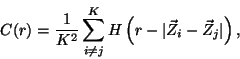
Let us generalize the above mentioned correlation integral (2) as following:

$$C(r)={1\over K^2} \sum_{i\not= j}^K H\left(r-\sqrt{\sum_{m=0}^{n- 1}(\vec{Z}_{i+m}-\vec{Z}_{j+m})^2}\right).$$

And one can define the quantity

$$H_2=\lim_{K\rightarrow \infty}\ln{C_n(r)\over C_{n+1}(r)}.$$

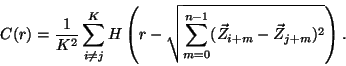
According to Ref. [4]:

$$H_2<H,$$

where $H$ is the Kolmogorov entropy.

The lower border of the Kolmogorov entropy has been measured for the Time Series of the $\delta$O$^{18}$ content in a deep-sea core. In Fig. 4 $H_2$ is plotted as a function of $n$ for two different values of $r$. As we see $H_2(n)$ reaches a saturation value $H_2=0.08$. And so, we can suppose that the Kolmogorov entropy of the climate system is not less than the value $H_2$.

The fact that the climate system has the positive Kolmogorov entropy value confirms that during last million years the climate evolution may be regarded as deterministic chaotic oscillation. It also means that the global climate changes may be predicted only in time, which is less than time $T$ [4]:

$$T\approx{1\over H}\ln\left({1\over l}\right)<{1\over H_2}\ln\left({1\over l}\right),$$

where $l$ is the initial state precision.

Acknowledgments

The author expresses his sincere thanks to Dr. S.N. Sergeev, without whom publication of this paper would not be possible.

Bibliography

1

N. Shackleton, N. Opdyke, Quat. Res. 3, 39 (1973)

2

M.I. Budyko, Changes of Climate, Gidrometeoizdat, Leningrad, 1972 (in Russian)

3

P. Grassberger, I. Proccacia, Phys. Rev. Lett. 50, 346 (1983)

4

H. Schuster, Deterministic Chaos, Physik-Verlag, Weinheim 1984

5

F. Takens, in: Lecture in Mathematics, Eds. D. Rand, B.S. Young, Springer, Berlin 1981, p. 898

6

N. Packard, J. Crutchfield, J. Framer, Phys. Rev. Lett. 45, 712 (1980)

7

A.S. Monin, Vvedenie v teoriu klimata, Gidrometeoizdat, Leningrad 1982 (in Russian)

This document was generated using the LaTeX2HTML translator Version 2K.1beta (1.47)
Copyright © 1993, 1994, 1995, 1996, Nikos Drakos, Computer Based Learning Unit, University of Leeds.
Copyright © 1997, 1998, 1999, Ross Moore, Mathematics Department, Macquarie University, Sydney.