|
|
|
Water nanodroplets in electrodynamic trap |
Electromagnetic trap
The hyperpoloidal Paul trap (Fig.1) creates a saddle-shaped oscillating electromagnetic field allowing for trapping a charged particle in the geometrical center of the trap. Such a field enables to trap dynamically a charged particle if the supplying voltage parameters (the frequency and the amplitude) were adjusted accordingly to the particle mass and charge.
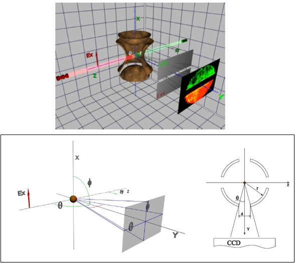
Fig. 1: Electromagnetic trap and observation geometry of light scattering experiment.
Droplet injector
Our droplet injector is a bubble-jet type device. We present it in figure We discharge a 10 µF capacitor charged to 250 V through a 7 mm resistive (kantal) wire - heater immersed in the liquid thus producing a pressure wave which ejects a single or few droplets through a special nozzle. We make nozzles of desired diameter by pulling, cutting and polishing of glass tube. It has been found that the wall thickness around the very nozzle should be considerable (several diameters of the opening) and the cone angle of the channel preceding the nozzle should be nearly right. The liquid is contained in a thick-walled tubular cuvette closed at one end with exchangeable nozzle and through the other end the power leads of the heater are introduced. There is a 3rd port in the middle pointing upwards through which the liquid is poured in. Droplets are injected through a 3 mm diameter port in the ring electrode. The injection timing is precisely controlled with a digital delay circuit utilizing the trap driving AC signal as the reference.
Climatic microchamber
The trap holder from the top and the droplet injector from the side are inserted into the ports of a double-walled air tight chamber - presented in figure 2 which can be cooled/heated with Peltier elements.
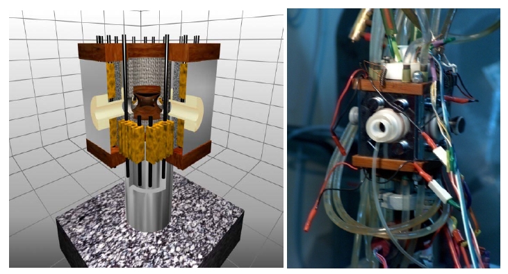
Fig. 2: Climatic microchamber.
Each Peltier element is in turn cooled with water. The cooling mechanism is quite efficient so that we can go below dew point in about 30 s and down to -30 C in several minutes. The bottom port can be used to control the pressure (vacuum pump) and the composition of the atmosphere inside the chamber. Thus we should be able to simulate the conditions and the dynamics of the upper troposphere. On the other hand heating and evacuating the chamber should enable us to get rid of unwanted liquid deposits (lost droplets) without taking out the trap.
Optical system
The chamber port and the 3 mm's diameter port in the trap ring opposite to the droplet injector are used for introducing the laser beams into the trap. The laser light polarization is 45 deg off vertical. This enables us to observe the scattered light at both p and s polarization geometries. As a matter of fact it also enables us to observe crossed polarizations ps and sp which can arise from nonsphericity of the droplet and thus measure such. CCD camera on the micromanipulator. Objective (compare main picture) and polarizer (inset). The scattered light is collected at right angle through another 3 mm's diameter port in the ring electrode with a microscope objective inserted into a chamber side port perpendicular to the injector and laser beam. The objective is characterized with a relatively large numerical aperture (DIN 10x, NA=0.3) though we do not use it along the DIN standard. The objective has been reassembled into a plastic body in order to suppress electrical and reduce thermal conductivity. The metal holder of the entrance lens which could not be removed has been equipped with a spring to provide electrical contact with the trap ring. This objective enables us to collect light from a cone of about 17 deg. Behind the objective, just in front of the CCD there are two semicircular sheet polarizers with polarization directions set perpendicularly dividing the field of view into two semicircles. This enables us to record scattering images on both polarizations simultaneously. The images are collected with a b/w CCD camera with gain control set to manual. The objective-camera system is set so that the object plane lies in front or behind the actual object (droplet). In this way we observe Mie interference patterns convoluted with the aperture rather than the surface of the droplet. Otherwise it would be impossible to resolve the fringes. The camera is placed on a micromanipulator so that we can measure its (relative) position with 0.1 mm precision. The images are digitized with a frame-grubber card for further processing.
|
Light scattering by microdroplets of water and
water suspensions |
-
Introduction
The observation of light scattered on various objects is a most common
method of investigation of the reality. In this paper we study the scattering
of light on water and water suspensions particle of the fundamental, ideal
shape of a sphere, with the radius comparable to the wavelength of the
used light a few micrometers. Under normal atmospheric conditions - below
100% relative humidity S - the droplets of pure water are not stable. They
grow for S>1 or shrink for S<1. Careful observation of light scattering
together with the appropriate use of theory allows to determine the radius
and the refraction index n (or dielectric function e:
e=n2)
of the droplet. The issue of refractive index is especially interesting
for droplets of suspensions, which are so omnipresent. In the first part
of this paper we present the study of evolution of pure water microdroplet
with well known refraction index. This investigation made it possible to
look into kinetic regime of droplet evolution - the region of droplet sizes
of the order of the free path of air molecules. In this region it is necessary
to supplement diffusion coefficient with so called evaporation coefficient
aC
describing
the ratio of the number of molecules crossing the liquid-vapor interface
to the number of molecules impinging on it: aC=nevap/ncol.
Similarly,
the thermal conductivity of moist air must be supplemented with the thermal
accommodation coefficient aT
determining
the probability that a molecule on impinging the interface attains the
thermal equilibrium with the medium on the opposite side. The literature
yields a very imprecise value for aC
and
aT
ranging from 0.01 to 1 (compare e.g.: [1, 2, 3, 4]). The
aim of our first experiments was to find the value of aC
and
aT
.
-
Model
The evaporation of droplets has been widely discussed, also taking
kinetic effects into account (see e.g.: [3, 4, 5, 6]). The evolution of
the droplet is driven by the gradients of temperature and water vapor density
near the droplet surface. However, water mass transport up to the distance
comparable to the mean free path of air molecules from the droplet surface
a<r<a+D
ought to be described with gas kinetic expressions (D
is of the order of the mean free path of air molecules [4]). For
r>a+D
the diffusional transport of the water vapor should be considered.
The droplet mass m change is equal to the flux of water through
the droplet surface:
 .
(1)  ,
,  , ,
(2)  , ,
(3)  , ,
(4)  . .
(5)  ,  ,
(6)
Thus, the model of evaporation utilized in our analysis consists of
two equations describing the transport of water mass (5) and heat (6) between
the droplet and its surroundings. Additionally we must remember about Rayleighs
condition [5] the fissility parameter X ought to be smaller
than 1:
 , ,
(7) It is worth noting that without the Rayleighs condition the equation
set (5)-(6) predicts the asymptotic stabilization of evaporating droplet
radius  for
a®aend,
given by the equation: for
a®aend,
given by the equation:
 . .
(8) -
Experiment
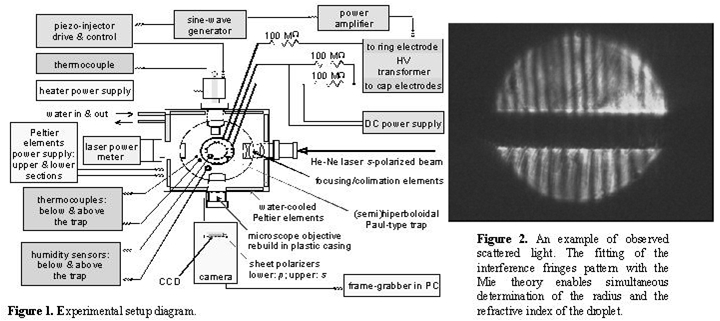
The experimental setup is presented in figure 1.
A detailed description can be found in our previous papers [7]. Paul trap
kept in the climatic microchamber is the heart of the system. Water droplets
are injected into the trap. The light scattered by the trapped particle
was collected through the port in the ring electrode with the microscope
objective positioned in the scattering plane at right angle from the direction
of the incident beams (see figure 2). The numerical aperture of the system
was ~0.17. The first experiments were conducted with pure water (20 ppb
total dissolved substances) at temperatures of 13.7 °C
and 13.1 °C, atmospheric pressure of 1006 hPa
and the charge Q of the order of 5´ 105
elementary charges. We registered the scaterograms of the evaporating droplet.
Then with the aid of the Mie theory the time dependence of droplet radius
was determined (see figures 3 and 4).
|
|
| Figure 3. Evaporation of
pure water droplet. |
Figure 4. Evaporation of
a contaminated water droplet. The stabilization of the radius for S<1
is possible due to the reduction of the vapor pressure over the curved
surface caused by the dissolved or surface active substances. |
From the time dependence of the radius a(t) we can determine
the value of the mass accommodation coefficient aC
=0.12±0.01, the thermal accommodation coefficient aT
= 0.65±0.09 as well as the very precise value of the relative humidity.
-
Local-field resonance in light scattering by a single
water droplet with spherical dielectric inclusions
In the second type of experiment we used the following suspensions
of nanospheres in water: (i) porous silica (refractive index
n=1.45)
of 300 and 450 nm diameter and (ii) polystyrene (n=1.58) of 200
nm diameter. Vertically polarized 632.8 nm He-Ne laser light was scattered
on a single levitated droplet of suspension. We registered the light scattering
patterns on s and p polarizations (perpendicular and parallel
to the scattering plane respectively) simultaneously. The signal in p
polarization appears when the levitated particle depolarizes light. Since
water was evaporating from the droplet, we could observe the transition
from scattering on a diluted suspension through scattering on a concentrated
suspension to scattering on a dry nanospheres agglomerate or a finite-size
highly imperfect photonic crystal. In the first case we observed a Mie
scattering pattern appearing on s polarization only (see figure
5a); the second (figure 5b) is characterized by a speckled Mie scattering
pattern and in the third (figure 5c) we can see bulk speckle or imperfect
Kossel lines [8] that are totally depolarized.
a
b
c
s-polarization 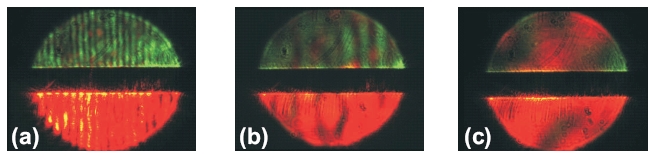
p-polarization
Figure 5. Examples of the scattering patterns observed
during evaporation of water from the droplet for low, medium and high concentration
of inclusions respectively.
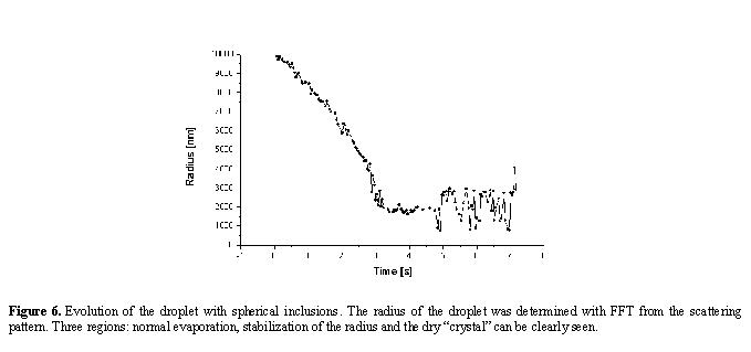
The spatial frequency of interference fringes for s light polarization
is nearly insensitive to the refractive index of the droplet while it exhibits
nearly linear dependence on its radius. It is then convenient to determine
the radius of the droplet with the aid of FFT [9]. In this way we obtain
the evolution of the droplet radius R(t) (see figure 6).
In the following part of this paper we use R instead of a
for effective radius of the particle, reserving a for inclusion
radius. On the other hand, the (averaged) intensity of the scattered light
Itot
depends on the effective index of refraction of the droplet meff.
We assume that for initial R the concentration of inclusions in
suspension is so small that we can put
meff=mw
(refractive index of water). This enables us to fix the scaling factor
of the fit. We ascribe all the variation of Itot to the
changes in the real part of
meff and we find meff
by fitting Itot with appropriately averaged Mie scattering
formulas. In figure 7 we present the results obtained for three experimental
cases, for three values of the radius of inclusion spheres and two types
of inclusion material.
 |
 |
 |
| Figure 7. The real part
of the effective dielectric function
eeff
as
a function of the droplet radius R for polystyrene inclusions of
a=200 nm, and silica inclusions of a=300 nm and a=450
nm. |
In order to further interpret the results we use the Lorentz effective
field theory, following Kreibig [10], but modifying the model slightly
and introducing the local field correction M(R). The effective
electric field of light at the position of a given inclusion can be expressed
as a Lorentz local field:
 ,
(10)  , ,
(11)  , ,
(12)   .
(13)  (Vinc
is the total volume of inclusions) enables to express the Lorentz-Lorenz
formula in the form proposed by Wiener: (Vinc
is the total volume of inclusions) enables to express the Lorentz-Lorenz
formula in the form proposed by Wiener:
 ,
(14)  .
(15)  ,
(16)
-
Light scattering analysis of water fullerene suspension
In the experiment of the third type we studied
light scattering at two wavelengths: red and green, on a droplet of water
fullerene (C60) suspension. We determined the evolution of the
droplet radius first. Two examples of such evolution are shown figure 8.
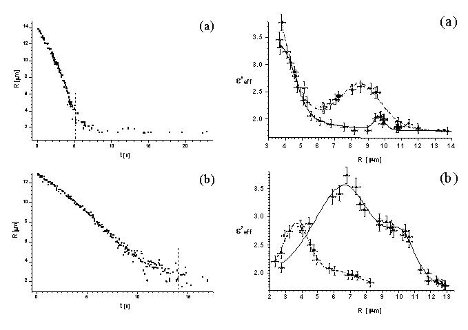
Figure 8. Left: the evolution of the radius of
C60 water suspension droplet, for high (a) and low (b) initial
fullerene contents. The vertical dashed lines show approximately the boundary
of wet particle region. Right: the real part of the effective dielectric
function of the composite droplet as a function of droplet radius; circles
and dash-dot line, green light scattering; triangles and solid line, red
light.
The experimental data effective dielectric function as a function
of radius - has been fitted with formulas (15) and (16) where
M(R)
accounted for two gaussian resonaces this time. The comparison of red and
green scattering allowed us to attribute these resonances to (diminishing)
average distance between neighboring scatterers (fullerene nanocrystallites).
We also tried to infer about the size of scatterers involved. For that
we needed Vincl which was known only for the case presented
in figure 8a, where the particle got completely dry. We assumed the aggregation
to be diffusion limited, though the aggregation scenario, is not fully
known. Elementary reasoning yields the radius of inclusion to be ~34 nm
in that case.
-
Conclusions
The elastic scattering of coherent light is a powerful tool for the
investigation of properties and structure of microdroplets. Careful analysis
of the scattered light enables to find the radius and refractive index
of the droplet and follow the evolution and evolution dynamics of these
quantities. Analysing the dynamics of the radius evolution and applying
a suitable thermodynamic model enables finding such parameters of the evolution
like mass and heat accommodation coefficients, pertaining to kinetic effects
manifesting for very small droplets. On the other hand studying the evolution
of effective refractive index, and utilizing a simple model, enables inferring
about the internal structure of the droplet of suspension as well as this
structure evolution.
| |
